A retrospective of NeurIPS 2020

I am going to begin with some practical things that I have taken away from NeurIPS this year. Careful setup and proper tuning of your models can make a big difference in performance. An amazing example of this are Steffen Rendle’s currently SOTA results for recommender ratings predictions on the Movielens 10M dataset, where a well tuned baseline is able to beat years of research on the topic.

Bag of tricks

Of course, setup and proper tuning is hard, so knowing current tricks for particular architectures, as well as how to combine them all together, is super useful. There are several bag of tricks summary papers that I know of for CNNs ^{1 2}, and I would love to hear about more. I found two more promising methods at NeurIPS this year that I will definitely try out.

Curriculum by Smoothing

Note

Suddenly, I found myself implementing convolutions in javascript. Anything to avoid writing? Use the slider to see the effect of annealing the standard deviation on the kernel and image.

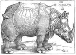
Curriulum learning is the idea of breaking a learning task down into units of progressively increasing difficulty, which is pretty much how humans learn. Curriculum by Smoothing ³ by Sinha et al proposes to apply this idea to CNN training. During early training, filters learned by the CNN will include high frequency data in the produced feature maps. These are details at very small scales. To illustrate the type of information we are talking about, let’s take a brief look at JPG compression:

Human vision has a drop-off at higher frequencies, and de-emphasizing (or even removing completely) higher frequency data from an image will give an image that appears very different to a computer, but looks very close to the original to a human. The quantization stage uses this fact to remove high frequency information, which results in a smaller representation of the image. ⁴

As it turns out, removing high frequency information during early training makes the learning problem easier. In this paper, high frequency data is removed at the beginning of training, and is exponentially annealed such that by the end of the training process, we are training on the original feature maps.

Annealing is done by reducing the variance of the gaussian kernel. This makes the gaussian more peaky and reduces the smoothing effect, until in the extreme case the kernel will have no effect at all. Have a play with the sidenote to see the effect.

The numbers presented in the paper look great 👏🏽. A resnet-18 baseline trained on imagenet obtains 68% top-1 accuracy, while using this training method the authors obtain 71% top-1 accuracy. Have a look at the paper for more details on transfer learning performance.

This work was done at the University of Toronto pair lab, and the github code provided by the very friendly lead author Sam Sinha is available here.

Hyperparameter search with ensembles of optimizers

I have never gotten far past random search when it comes to automated tuning of hyperparameters. I suppose that effective hyperparameter tuning continues to be a matter of experience ⁵, hat tip to Henry from dragonfly for pointing out this paper.

Nevertheless, I always wondered what some of the cloud hyperparameter tuning offerings cloud could do. Thanks to the NeurIPS black box optimization challenge, which ran as part of the competitions programme, I might have something new to try out myself instead. Results can be seen on the leaderboard, along with papers and code for some of the contestants.

My main takeaway is that large improvements could be made to off-the-shelf black box optimisers through ensembling of readily available open source implementations. This paper by Nvidia RAPIDS ⁶ found that combining Turbo with either Hyperopt or Scikit Optimize yielded good results.

Accountability

For me, this was the year that the broader impact of AI is truly being seen and addressed by the community. You can’t just hide out in your workplace, tuning hyperparameter while ignoring developments in the world at large. This wonderful keynote on the topic by Charles Isbel is worth your time:

Successful technological fields have a moment when they become pervasive, important, and noticed. They are deployed into the world and, inevitably, something goes wrong. … The field must then choose to mature and take responsibility for avoiding the harms associated with what it is producing. Machine learning has reached this moment.

I do think the tone here is telling, and that many in the field still refuse to think about their personal accountability. It is something I would like to think about a lot more in 2021.

Systems out there are already making life changing decisions for potentially vulnerable people, without providing any path to recourse. However, being able to explain your predictions is an important part of providing recourse for your system.

Next up, a tutorial on explaining machine learning predictions.

Two paths towards explainable systems are to either make the system inherently explainable, or to provide post hoc explanations of black box systems.

Explainable models

The easiest way to obtain explanations for your model is to start with a model that is already explainable. Generalised additive models, described by Hastie and Tibshirani in the early 90’s, are one such model. Here is the formulation for regression:

$\mathbb{E}(Y|X_1, X_2, ..., X_p) = \alpha + f_1(X_1) + f_2(X_2) + ... + f_p(X_p)$

The functions $f$ can be directly inspected after learning.

This glassbox model has recently popped up in various places, including Rich Caruna’s EMNLP keynote a few weeks ago. It is one of a family of algorithms ⁷ that can be readily interpreted. As an aside, Rich Caruna’s group has brought GAMs into the world of deep learning ⁸, in the hopes of kickstarting research into glassbox deep learning. The model simply sums over $p$ independent feed forward networks that respectively process one feature at a time. Code is available here, tweetprint here.

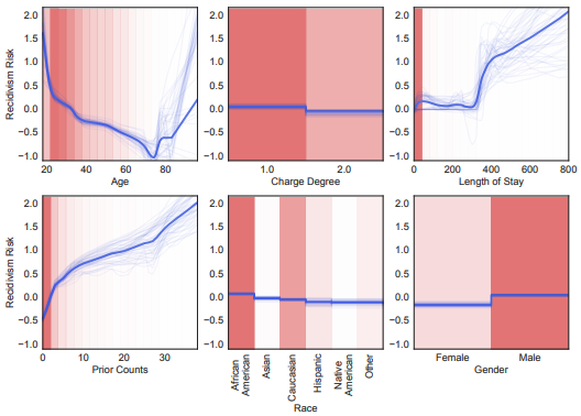
Here we see the risk of re-offence for released prisoners. The shape function for race suggests that the learned model is racially biased: black defendants are predicted to be higher risk for reoffending than white or Asian defendants.

See the paper ⁸ for full details.

Another method is to train a more powerful black box model, and then to use model distillation to train a student glassbox explainer model.

Post hoc explanations

The tutorial was however largely focussed on post hoc explanations. These treat the model as a black box. Explanations are developed around usually deep models.

Post hoc explanations come in two flavours: local and global. Local explanations seek to exlain single examples, e.g. why a single image was classified as a wolf. Global explanations seek to explain models in their aggregate behaviour, e.g. in order to expose systematic bias in the model.

Local explanations can be understood as zooming into a single example and looking at the decision boundary closest to that example. One family of local explanations determines which features are important in the prediction for the given example.

Lime ⁹ seeks to generate a sparse linear approximation of the local decision boundary. As many features as possible are zeroed out in order to identify the important dimensions, and the regression encodes the relative importance of those remaining features. This way, we can determine which features are important in the prediction for the given example.

As described in the paper, the original decision function $f$ (unknown to LIME), cannot be approximated well by a linear model. The blue circle is the instance being explained. LIME samples instances, gets predictions using $f$, and weighs them by the proximity to the instance being explained (represented here by size). The straight line is the learned explanation that is locally (but not globally) faithful; hover to see the effect.

LIME requires us to decide a bunch of things. First, we have to find some way to perturb instances around the example we are examining. For an automatic speech recognition system, we might remove certain frequencies, or perturb the input audio in high level ways. Then we have to have to determine a distance function to measure how far away we are from the example we are examining. We could also choose different feature representations – e.g. pixels, or superpixels. All these decisions introduce a large number of hyperparameters that affect how we should understand the explanation.

Shap ¹⁰, like LIME, perturbs examples and measures the importance of individual features for a prediction. The main difference is that the marginal contribution of each feature is calculated. This is done by looking at all possible permutations of features, e.g. all possible images, and calculating the probability of each instance, then the probability with the feature in question turned off. The average of all these marginal contributions is the shapley value for this feature. This method is grounded in game theory, and provides guarantees about the fair attribution of the prediction to all features. Of course, we’ll have to find some sampling approximations. There’s a lot to unpack here, and I plan to spend some time on reading the paper and understanding the theory of shapley values.

Much more in the interest of actually finishing this post, I will stop here. Have a look at the tutorial, the rest is really the most interesting material. The use of counterfactuals to create actionable model explanations is really interesting, and there is a host of other valuable explainers.

Model compression

Three methods seem to have come together to allow for extreme compression of models. Compression seeks to both reduce the size of models, and to increase the speed at which inference can be done such that CPU inference becomes feasible. Large energy and cost savings can also be realised using these methods, thereby reducing the lifetime environmental impact of the model. In some cases, it may not even be possible to deploy models directly to mobile devices without compression.

FastFormers ¹¹, through carefully utilizing knowledge distillation, structured pruning and numerical optimization, can lead to drastic improvements on inference efficiency. This particular model is on top of Hugging Face’s BERT and RoBERTa, and is currently being added to Hugging Face Transformers.

Sparsification is about removing vertices or edges in the network. Despite the paper above, unstructured pruning, the removing of connections, seems to often works better than structured pruning, which is when whole neurons are removed. Gradual magnitude pruning appears to be the method of choice in practice ¹². Starting with a trained network the weights closest to zero are iteratively removed over several epochs. A detailed guide to pruning with GMP can be found here. Current literature reviews are available from Google ¹³ and MIT ¹⁴.

Quantisation ¹⁵ is the process of compressing model weights. I have recently switched to mixed precision wherever I can, which reduces the weights from 32 bits to 16 bits of precision. Quantisation switches to integers, and routinely reduces these down to 8 bits. I was amazed to learn that you can even take it down to 2 bits while still retaining a reasonably degraded model performance. I was not aware that pytorch natively supports int8 quantisation, including inference via fbgemm. Some recent ¹⁶ work ¹⁷.

Distillation ¹⁸ is about training a smaller student model that is often able to match the performance of the teacher model. See TinyBERT ¹⁹ for an example of distillation in NLP.

🤗 Hugging face

Speaking of Hugging face, there was a nice talk on it by the very tired Tom Wolf . The Transformers library is up to an amazing 40 models with checkpoints. I did not know that hugging face now includes a very nice and fast growing collection of NLP datasets. As easy as:

from datasets import load_dataset
dataset = load_dataset("librispeech_lm")

One interesting thing he said related to limits of the current generation of language models. Language datasets do not include things that are trivially obvious to us. For example, we will not describe a sheep as white. If you were to look for sheep colors in written language, you might very well be led to believe that sheep are predominantly black. This effect is investigated in Van Durme et al ²⁰.

A possible solution, discussed by Tom, is to use embodied language datasets. That is, speech including video and or images. If you have people speaking about things that can be seen, then we can try to derive the obvious facts from there.

Self-supervised learning for audio and speech

The NeurIPS Workshop (also here) on self-supervised learning for audio and speech was held on the last day of the conference. These were my highlights.

Wav2vec 2.0

One of the key papers for me this year was Wave2vec 2.0 ²¹, which leverages self-supervised pretraining for automatic speech recognition. The approach is able to drop word error rates down to 1.8% in certain settings. See the poster session video here, code here.

A large unlabelled dataset is used to pretrain a model, and this is then leveraged for a supervised downstream task with a potentially small labelled dataset. Applied to automatic speech recognition, it opens up better performance in low resource settings. In a low resource setting where we only have 100 hours of labelled speech, using the base model with 100MM parameters, we can obtain a WER of 7.8.

The model processes raw audio $\mathcal{X}$ with stacks of CNNs. The resulting representation $\mathcal{Z}$ is partially masked and sent through a transformer to obtain a low frequency high level representation $\mathcal{C}$, which is contextualised by information to both the left and right. Independently, $\mathcal{Z}$ is quantised into a low dimensional discrete representation $\mathcal{Q}$. This is not passed through the transformer.

To complete the model, we need to define the pretext task. The point of this task is to produce good representations of the data. We could be predicting a masked word in a sequence, as in word2vec or BERT and friends. In this work, the pretext is to find the correct speech representation at a masked location. Instead of predicting the whole representation, the task is to find it hidden in a set of distractors.

Masking for the transformer input, we’re going to use a masked language modelling approach, and replace around 50% of the data with a mask. In this case, the mask is a learned vector. This also means that only around half of the batch is contributing to the loss at any given time. Masking is happening on the low frequency (~50hz) $\mathcal{Z}$ representation, and spans of size 11 will be masked, which translates to around 230ms of audio at a time. Due to the sampling strategy spans may collapse into larger spans. Masking should occur once at the dataset level to avoid information leakage.

This is where $\mathcal{Q}$ comes into the picture: the prediction $c_t$ at this timestep is projected against each of the sampled distractors $\tilde{q}$, and we would like to maximise the inner product between $c_t$ and $q_t$, while minimizing it with distractors. Given that $sim(a, b)$ is defined to be the cosine similarity, the contrastive loss or this task looks like this:

This is also known as the NT-Xent loss ²⁴, the normalized temperature-scaled cross entropy loss. The loss is calculated only on each masked output timestep $c_i$, using only distractors $\tilde{q}$ that were not visible to the transformer.

Once the pretraining has been completed, a linear layer is added to the top of the network, and is trained with a CTC ²² loss against phone or letter unaligned ground truth.

Key elements of the model:

• Bi-directional contextualised representations
• Contrastive task
• Vector quantised targets
• Fine tuned on labelled data

DeCoAr 2.0

Flexible contextualized speech representations for downstream tasks by Katrin Kirchhoff presents work done by AWS AI that has many similarities to Wave2vec 2.0. Like above, we have a transformer, quantised representations, and pretraining on raw audio. But the framing for DeCoAr 2.0 ²³ is a bit different – users should be able to use the representations as is, without finetuning. That is, the model is frozen on the downstream task, and only the top layer is retrained.

Also, while the loss in Wav2vec 2.0 is discriminative, DeCoAr 2.0 uses a reconstructive loss. Again, certain spans are masked, but the task is to fully reconstruct those spans. The reasoning here is that for a discriminative loss, you need to think carefully about the strategy you use to sample negatives, as this has a large effect on the representations you are learning. So for different downstream tasks, you may need to adjust your negative sampling strategy. In this work, the authors are trying to learn representations that work, as they are, on many different downstream tasks.

Multiformat contrastive learning

Multiformat contrastive learning of audio representations ²⁵ is another interesting work, by Lyu Wang and Aäron van den Oord . It claims a 32% relative improvement by introducing two audio formats to the contrastive task. Instead of just using the waveform, they use both the raw waveform and a log mel filterbank representation.

The surprising thing here is that large gains are to be had by encoding the same modality in two different ways. When using two modalities, e.g. audio and video, one might expect that the complementary data will lead to improvements. Why this is the case with the same modality is an open question.

The model is based on SimCLR ²⁴, and looks as follows.

Augmentations for the raw waveform include time masking and taking another example from the batch, multiplying it by a small number and adding it in to simulate noise. For the spectogram we can do the same, but also do frequency masking and shifting. To train, the positive pair is the one generated by the same underlying example, while the negative pairs are generated by the other examples in the same batch. The NT-Xent loss described above is used, except that $sim(a, b)$ uses a learnable function $g$, a linear MLP, on top of the normalised representations.

Note that because we are taking negatives from the same batch, the batch size has a large effect on this method. It seems that you might need crazy large batch sizes like ☄️ 32K to make this work well. I haven’t looked at how much memory you need on your GPUs to fit these batches.

Beyond masked language modelling

Denoising of seq2seq pre-training was presented by the cheerfully self-deprecating Luke Zettlemoyer of FAIR, slides here. It turned out to be an unexpected walk through the world of the BERT ecosystem, as well as a discussion of what really works in self-supervised pretraining here. While a lot of this may be familiar to people, I found it quite enlightening.

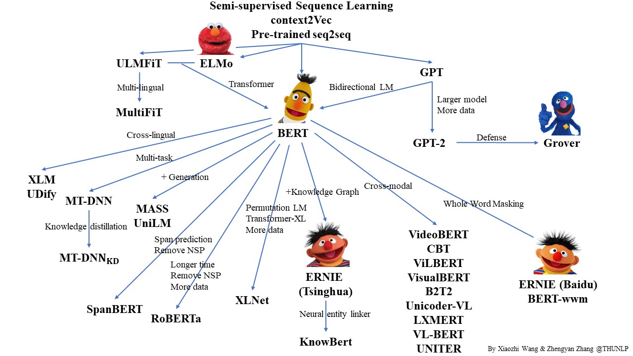
BERT ²⁶ is the something like the Abraham of this ecosystem, while building on previous pretraining results. It was published in 2018, and at the time it obtained SOTA results on 11 different natural language processing tasks. The basic setup is a transformer model with bidirectional context which is pretrained with a masked language modelling loss – that is, 15% of words in the training data are replaced with a <MASK> token, and the task is to predict these tokens. In each batch, only the <MASK> tokens contribute to the loss.

RoBERTa ²⁷ is a scaled up and somewhat tighter version of BERT, and Luke Zettlemoyer is one its authors. In the original BERT model, two sentences are always passed into the model side to side. The aim was to create a general model that can also be used for question answering, and so BERT includes a discriminative sentence level loss term to check if the following sentence is correct or not. RoBERTa does away with this, adds more data, and increases batch size and compute.

These two bidirectional masked language models are quite powerful classifiers, but when it comes to generation, autoregressive or causal losses are standard, as in the GPT family.

Bart ²⁸ is a consolidated model that can be used both for classification and generation. The trick here is to frame the task as a seq2seq model, and to view the encoder-decoder pair as a denoiser. The nice thing about this model is that by changing the noising function, it can accommodate many different methods within a single framework.

The encoder is bidirectional, while the decoder attends to all of the timesteps of the encoder and is causally directed. In this case, a masked language model objective has been used. Some possible noising functions:

• Masking
• Deletion
• Document rotation – a document level task
• Sentence permutation – recreate original order
• Text infilling – delete multiple words but only provide one mask token

As it turns out, text infilling is the most effective noiser. Span lengths are drawn from a poisson distribution, and could be zero length. Bart appears to be particularly good at summarization.

Retrieval Augmented Generation ²⁹, which was also presented at the conference, is a nice retrieval application of Bart. RAG combines different methods into a larger end-to-end architecture. Here, we can combine the virtues of Bart – powerful bidirectionally contextualised language representations for retrieval, a causal generator for generation, and strong performance on many tasks.

Here’s the model:

We combine a pre-trained retriever (Query Encoder + Document Index) with a pre-trained seq2seq model (Generator) and fine-tune end-to-end. For query $x$, we use Maximum Inner Product Search (MIPS) to find the top-K documents $z_i$. For final prediction $y$, we treat $z$ as a latent variable and marginalize over seq2seq predictions given different documents.

I invite you to try RAG for yourself. Install the dependencies:

conda create --name rag
conda activate rag
conda install pytorch faiss-cpu -c pytorch
conda install -c huggingface transformers
pip install datasets

We can load a sample of wikipedia dpr and ask questions about it. Running this will lazily download around 8GB of data:

from transformers import RagTokenizer as Tok
from transformers import RagRetriever as Ret
from transformers import RagTokenForGeneration as Gen
model = 'facebook/rag-token-nq'
index = {
  'index_name': 'exact',
  'use_dummy_dataset': True
}
t = Tok.from_pretrained(model)
r = Ret.from_pretrained(model, **index)
g = Gen.from_pretrained(model, retriever=r)
def rag(q):
  inp = t.prepare_seq2seq_batch(q, return_tensors='pt')
  out = g.generate(input_ids=inp['input_ids'])
  return t.batch_decode(out, skip_special_tokens=True)[0]

Now you can ask questions like 'when was taika waititi born' – but don’t get excited quite yet:

rag('who has the record in 100m freestyle') => 'michael phelps'
rag('who is hedwig') => 'ask the host'
rag('who is michael phelps') => 'michael phelps'
rag('what color is an apple') => ''
rag('when was richard nixon born') => '1969'
rag('when was taika waititi born') => 'in may 2000'

It looks like more work is needed to get an example running well.

mBart ³⁰ uses Bart pretraining for a downstream translation task. Here, the idea is to train as above, but mixing together instances from different languages. Once pretraining is done, a bi-text dataset is used for supervised finetuning using the same seq2seq model and loss. This looks quite promising for middle and low resource language pairs, although anything with less than 10K examples does not appear to be fine tunable. mBart can be used together with back translation. The idea here that you start with weak model and a monolingual corups, and then use the predictions as ground truth to retrain on. This is done over many iterations.

New Zealand 🥝

I’ve been in Wellington, NZ for a while, and recently got introduced to some local machine people by the very nice Tom Barraclough of Brainbox, who is doing interesting work at the intersection of legal tech and citizen empowerment. One these people was Caleb Moses of Dragonfly Data Science.

Indigenous in AI

Caleb drew my attention to the Indigenous in AI workshop, which he co-organised at NeurIPS this year. He is part of a group of technologists working with Te Hiku Media to build speech technology for Te reo Māori. The keynote by Peter-Lucas Jones CEO of Te Hiku Media and CTO Keoni Mahelona introduced the challenges and positions of Māori Iwis in a compelling way. In their words:

Te Reo Irirangi o Te Hiku o Te Ika (Te Hiku Media) is a non-profit organisation whose mission is to preserve and promote te reo Māori, the indigenous language of New Zealand. Over the past 30 years we’ve recorded thousands of hours of the stories of our people, most of whom were native speakers. These stories are rich in culture and traditional knowledge around science, the environment, and traditional Māori medicine. Today, we operate in digital industries creating technology to help document, conserve, and share the language and knowledge in novel ways. Central to the development of technology and the collection of data is the formalisation of our cultural practices into our Kaitiakitanga License . The license outlines the way that people are able to access data gathered and acknowledges the value of open source technologies but recognises the impact of colonisation on indigenous peoples’ ability to access those technologies. This discussion will provide insight into the Kōrero Māori project and its progress to date in creating speech to text, text to speech, and pronunciation tools. We demonstrate how innovation in language revitalisation succeeds when an indigenous organization leads the corpus collection and technology development. We collected more than 300 hours of labeled corpus in ten days. This enabled the creation of an automatic speech recognition (ASR) tool for te reo Māori using Mozilla’s DeepSpeech project with a word error rate of 14%. The ASR tool is being used to speed up the transcription of our native speaker archives. FN

Have a listen to this interview and the Indigenous AI position paper to learn more.

The end 🎬

All in all, remote NeurIPS was a success for me, and I enjoyed it a lot. There are a bunch of sessions I would still like to have a look at in the coming weeks. In a note to myself, my most missed workshops. Note that these these will become available to non-attendees at the end of January:

• ML for creativity and design. Lots of interesting applications here.
• Tackling climate change with ML. Power plant emissions estimates from satellite data 🔥
• Resistance AI. Important. Regret missing this.
• Self-supervised learning. Theory and practice, definitely want to catch up on this.
• Meta learning. Seems like everybody is talking about meta learning. Best have a look.
• Beyond backprop. Intriguing. Looks like a lot of research directions here.

Most missed Tutorials:

• Practical uncertainty estimation and OOD robustness. With Dustin Tran. Looks 🔥
• Abstraction and reasoning in AI Francois Chollet on better benchmarks. Looks important.
• Neural ODEs. Saw this done in Julia before, want to learn more.

Sign up to the FELD newsletter👇🏽 below

If you liked this post and would like to read more like this, sign up to the newsletter! I enjoyed writing this, and since I have now finally set up the blog properly I intend to publish as often as I can. See you soon 👋

References